PAW All-Electron Wavefunction in VASP

Introduction

In the PAW method, the all-electron (AE) wavefunction (AEWFC) $ψ_{n k}$ is related to the pseudo-wavefucntion (PSWFC) ${\tilde{ψ}}_{n k}$ by means of a linear transformation ¹

\begin{matrix} (1) & | ψ_{n k} ⟩ = | {\tilde{ψ}}_{n k} ⟩ + \sum_{j} [| ϕ_{j} ⟩ - | {\tilde{ϕ}}_{j} ⟩] \cdot ⟨ {\tilde{p}}_{j} | {\tilde{ψ}}_{n k} ⟩ \end{matrix}

**Figure 1.** Compositions of the all-electron wavefunction within the PAW method.

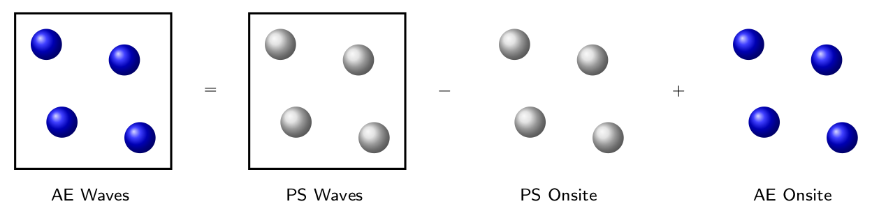
Note that both AEWFC and PSWFC are defined on the Born-von Kármán (BvK) supercell rather than the unit cell, therefore, the index j in Eq. $(1)$ depends not only on the atom index in the unit cell but also on the index of the unit cell, i.e.

\begin{matrix} (2) & \sum_{j} ⟹ \sum_{R_{L}} \sum_{τ_{α}} \sum_{k} \end{matrix}

The forms of the projector function $\tilde{p}$ , and the partial waves $ϕ$ and $\tilde{ϕ}$ , however, are only determined by the kind of the atom except that the centers depend on the cell and atom indices.

AEWFC and PSWFC

The AEWFC $ψ_{n k}$ and the PSWFC ${\tilde{ψ}}_{n k}$ both take the form of a Bloch wave, i.e.

\begin{aligned} (3) & | ψ_{n k} ⟩ & = e^{i k \cdot r} \cdot | u_{n k} ⟩ \\ (4) & | {\tilde{ψ}}_{n k} ⟩ & = e^{i k \cdot r} \cdot | {\tilde{u}}_{n k} ⟩ \end{aligned}

where $u_{n k}$ and ${\tilde{u}}_{n k}$ are cell-periodic functions.

In VASP, cell-periodic part of the PSWFCs, i.e. $| {\tilde{u}}_{n k} ⟩$ , are the ones included in the WAVECAR file, only that the plane-waves coefficients $C_{n k} (G)$ are written instead.

\begin{aligned} C_{n k} (G_{j}) & = \int {\tilde{u}}_{n k} (r) \cdot \frac{1}{\sqrt{V}} e^{- i G \cdot r} d r \\ = \sum_{k} {\tilde{u}}_{n k} (r_{k}) \cdot \frac{1}{\sqrt{V}} e^{- i G_{j} \cdot r_{k}} Δ V \\ (5) & = \frac{V}{N_{fft}} \sum_{k} {\tilde{u}}_{n k} (r_{k}) \cdot \frac{1}{\sqrt{V}} e^{- i G_{j} \cdot r_{k}} \\ (6) & {\tilde{u}}_{n k} (r_{j}) & = \sum_{k} C_{n k} (G_{k}) \cdot \frac{1}{\sqrt{V}} e^{i G_{k} \cdot r_{j}} \end{aligned}

where $N_{fft}$ is the number of FFT grid points, $V$ is the cell volume, and the plane-waves are limited within the sphere defined by

\begin{matrix} (7) & \frac{ℏ^{2} | G + k |^{2}}{2 m_{e}} < E_{c} \end{matrix}

The relation between the norm of ${\tilde{u}}_{n k} (r)$ and $C_{n k} (G)$ are given by the following equation

\begin{matrix} (8) & \sum_{G} | C_{n k} (G) |^{2} = \frac{V}{N_{fft}} \sum_{r} | {\tilde{u}}_{n k} (r) |^{2} \approx 1 \end{matrix}

Note that the norm of the PSWFC can be larger or smaller than one, hence we use “ $\approx$ ” instead of equal sign in the above equation.

To obtain the real-space representation of ${\tilde{u}}_{n k}$ , one need to perform Fourier transform (FT) on the plane-wave coefficients, which can be easily realized utilizing the VaspBandUnfolding package.

The real-space representation of $u_{n k}$ is not as readily obtainable, since it contains the on-site contributions that are defined on multiple radial logarithmic grids with different centers, which are not compatible with the uniform grid used to represent ${\tilde{u}}_{n k}$ .

Projector Function

The projector functions ${\tilde{p}}_{j}$ depend on the distance from the center of the PAW sphere on which they are localized,

\begin{matrix} (9) & ⟨ r | {\tilde{p}}_{j} ⟩ = {\tilde{p}}_{j} (r - R_{L} - τ_{j}); | r - R_{L} - τ_{j} | < r_{j}^{c} \end{matrix}

where $r_{j}^{c}$ is the PAW sphere cutoff radius, $R_{L}$ is the cell vector of the L-th unit cell and $τ_{j}$ is the atom position within the cell.

Note in passing that $r_{j}^{c}$ in VASP does not necessarily satisfy the non-overlaping condition. For examples, $r_{O}^{c} = 0.82 \overset{˚}{A}$ and $r_{H}^{c} = 0.59 \overset{˚}{A}$ while a typical O-H bond length is about $0.97 \overset{˚}{A}$ .

For simplicity, we only consider the projector functions located within the first unit cell, i.e. $R_{0} = (0, 0, 0)$ . The form of the projector function is composed of a radial part and an angular part, i.e.

\begin{matrix} (10) & {\tilde{p}}_{j} (r - τ) = f_{j} (| r - τ |) \cdot Y_{l m} (\hat{r - τ}) \end{matrix}

where REAL FUNCTION $f_{j} (r)$ and real spherical harmonics $Y_{l m}$ are used in order to save computational cost. The Fourier transform of the projector function, as is shown in a previous post,² can also be written as a radial function multiplied by a real spherical harmonics with the same $(l, m)$ quantum numbers, i.e.

\begin{aligned} (11) & F [{\tilde{p}}_{j} (r - τ)] (k) & = \frac{1}{\sqrt{V}} \int_{V} {\tilde{p}}_{j} (r - τ) e^{- i k \cdot r} d r \\ (12) & = \frac{i^{- ℓ}}{\sqrt{V}} \cdot g_{j} (k) \cdot Y_{l m} (\hat{k}) \cdot e^{- i k \cdot τ} \end{aligned}

where the phase term is due to the shifting property of FT. $f_{j} (r)$ and $g_{j} (k)$ are linked by spherical Bessel transform,³

\begin{matrix} (13) & g_{j} (k) = 4 π \int_{0}^{\infty} f_{j} (r) j_{l} (k r) r^{2} d r \end{matrix}

Obviously, $g_{j} (k)$ is also a REAL FUNCTION by definition.

In VASP, the information of the projector functions are included in the POTCAR file, however, only radial parts of the real- and momentum-space projector functions, i.e. $f_{j} (r)$ and $g_{j} (k)$ , are are stored. As a result, one must multiply the radial function with the corresponding real spherical harmonics $Y_{l m}$ in order to get the complete projector function.

**Figure 2.** Upper panels: radial parts of the projector functions in real (left) and momentum (right) space for Ti POTCAR. The vertical dashed lines in the left and right panels correspond to the real- and reciprocal-space cut, respectively. Lower panel: radial parts of the AE and PS partial waves on the logarithmic radial grid, shown with solid/dashed lines, respectively. The figure was generated with the potplot script.

To evaluate the inner-product of the projector function and PSWFC, an extra k-dependent projector function ${\tilde{p}}_{j k}$ is introduced in VASP⁴

\begin{matrix} (14) & | {\tilde{p}}_{j k} ⟩ = e^{- i k \cdot (r - τ_{j})} \cdot | {\tilde{p}}_{j} (r - τ_{j}) ⟩ \end{matrix}

As a result, the inner product between the projector and PSWFC can be written as

\begin{aligned} (15) & β_{n k}^{j} & = ⟨ {\tilde{p}}_{j} | {\tilde{ψ}}_{n k} ⟩ \\ (16) & = e^{i k \cdot τ_{j}} \cdot ⟨ {\tilde{p}}_{j k} | {\tilde{u}}_{n k} ⟩ \\ (17) & = e^{i k \cdot τ_{j}} \cdot β_{n k}^{j k} \end{aligned}

Note that in practical implementation,VASP DOES NOT include the phase term $e^{i k \cdot τ_{j}}$ in the actual calculation, since it does not change the occupation matrix or energy, as is explained in the nonl.F of VASP source file.

One can clearly see from Eq. $(17)$ that for the same projector function located at another unit cell $R_{L}$ , the inner product is simply right-hand-side of Eq. $(17)$ multiplied by $e^{i k \cdot R_{L}}$ .

With this definition, Eq. $(17)$ can be evaluated in two different approaches:

momentum-space method

\begin{aligned} ⟨ {\tilde{p}}_{j k} | {\tilde{u}}_{n k} ⟩ & = \sum_{G} ⟨ {\tilde{p}}_{j k} | G ⟩ ⟨ G | {\tilde{u}}_{n k} ⟩ \\ = \sum_{G} ⟨ {\tilde{p}}_{j} (r - τ_{j}) | e^{i k \cdot (r - τ_{j})} | G ⟩ ⟨ G | {\tilde{u}}_{n k} ⟩ \\ = \sum_{G, G^{'}} ⟨ {\tilde{p}}_{j} (r - τ_{j}) | G^{'} ⟩ ⟨ G^{'} | e^{i k \cdot (r - τ_{j})} | G ⟩ ⟨ G | {\tilde{u}}_{n k} ⟩ \\ = e^{- i k \cdot τ_{j}} \cdot \sum_{G, G^{'}} ⟨ {\tilde{p}}_{j} (r - τ_{j}) | G^{'} ⟩ δ_{G^{'}, G + k} ⟨ G | {\tilde{u}}_{n k} ⟩ \\ = e^{- i k \cdot τ_{j}} \cdot \sum_{G} ⟨ {\tilde{p}}_{j} (r - τ_{j}) | G + k ⟩ ⟨ G | {\tilde{u}}_{n k} ⟩ \\ = \frac{e^{- i k \cdot τ_{j}}}{\sqrt{V}} \sum_{G} i^{l} g_{j} (| G + k |) Y_{l m} (\hat{G + k}) e^{i (G + k) \cdot τ_{j}} \cdot C_{n k} (G) \\ (18) & = \frac{1}{\sqrt{V}} \sum_{G} i^{l} g_{j} (| G + k |) Y_{l m} (\hat{G + k}) e^{i G \cdot τ_{j}} \cdot C_{n k} (G) \end{aligned}

In the first step, one has to find out all the plane-waves within the sphere defined by Eq. $(7)$ . Secondly, $g_{j}$ values on the relevant $| G + k |$ are obtained by Spline-interpolation and multiplied with the corresponding real spherical harmonics $Y_{l m}$ . The sum over $G$ can then readily obtained with the knowledge of the plane-wave coefficients.

Note that this is what VASP does by setting LREAL = .F. in the INCAR.

real-space method

\begin{aligned} ⟨ {\tilde{p}}_{j k} | {\tilde{u}}_{n k} ⟩ & = \int_{| r - τ_{j} | < r_{j}^{c}} e^{i k \cdot (r - τ_{j})} \cdot f_{j} (| r - τ |) \cdot Y_{l m} (\hat{r - τ}) \cdot {\tilde{u}}_{n k} (r) d r \\ (19) & = \sum_{| r_{k} - τ_{j} | < r_{j}^{c}} e^{i k_{k} \cdot (r - τ_{j})} \cdot f_{j} (| r_{k} - τ_{j} |) \cdot Y_{l m} ({\hat{r_{k} - τ}}_{j}) \cdot {\tilde{u}}_{n k} (r_{k}) \cdot \frac{V}{N_{fft}} \end{aligned}

First, the grid points within the PAW sphere $| r - τ_{j} | < r_{j}^{c}$ are identified. Secondly, the values of $f_{j}$ on these grid points are obtained by Spline-interpolation and multiplied with the corresponding real spherical harmonics $Y_{l m}$ . Finally, muliplying the phase term and ${\tilde{u}}_{n k} (r)$ , the integral becomes a sum over the selected grid points.

Note that this is what VASP does by setting LREAL = .T. in the INCAR.

Partial Waves

The AE/PS partial waves $ϕ_{j}$ and ${\tilde{ϕ}}_{j}$ are defined on the radial logarithmic grid with center at $τ_{j}$ (in the first unit cell), i.e.

\begin{aligned} (20) & ⟨ r | ϕ_{j} ⟩ & = ϕ_{j} (r - τ_{j}) \\ (21) & ⟨ r | {\tilde{ϕ}}_{j} ⟩ & = {\tilde{ϕ}}_{j} (r - τ_{j}) \end{aligned}

The radial logarithmic grid is defined as

r_{n} = r_{0} \cdot e^{n \cdot H}; n = 0, 1, 2, \dots, N - 1

or equivalently

r_{n + 1} = r_{n} \cdot e^{H}; n = 0, 1, 2, \dots, N - 1

where $r_{0}$ is the minimum value of $| r - τ_{j} |$ and is by definition not zero, $N$ is the number of radial grid points.

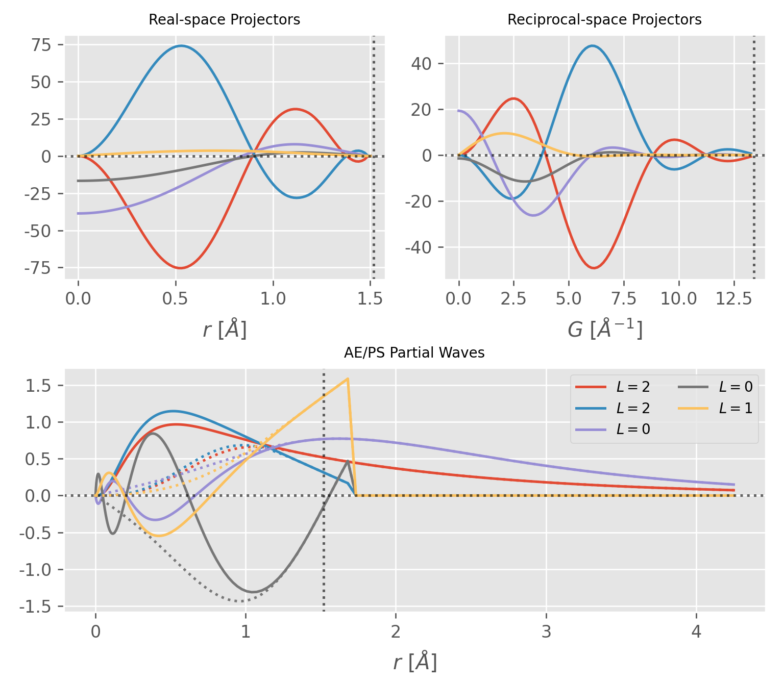
Note that $r_{N - 1}$ is not necessarily equal to the PAW sphere cutoff radius $r_{j}^{c}$ , as can be seen in Figure 2. However, $ϕ_{j}$ and ${\tilde{ϕ}}_{j}$ are indential beyond $| r - τ_{j} | = r_{j}^{c}$ , which makes the difference of the two zero in Eq. $(1)$ beyond $r_{j}^{c}$ .

The AE/PS partial waves are again composed of radial and angular parts,

\begin{array}{r} (22) & ϕ_{j} (r - τ_{j}) = \frac{R_{j} (| r - τ_{j} |)}{| r - τ_{j} |} \cdot Y_{l m} (\hat{r - τ_{j}}) \\ (23) & {\tilde{ϕ}}_{j} (r - τ_{j}) = \frac{{\tilde{R}}_{j} (| r - τ_{j} |)}{| r - τ_{j} |} \cdot Y_{l m} (\hat{r - τ_{j}}) \end{array}

IT MUST BE STRESSED that $R_{j} (r)$ and ${\tilde{R}}_{j} (r)$ are the ones stored in the POTCAR file and are also the ones shown in Figure 2.

A few notes on the construction of AE/PS partial waves

The AE partial waves are chosen to be solution to Schrödinger equation for a fixed quantum number l and chosen reference energy. ⁵
The PS partial waves are, by definition, indential to the AE partial waves outside th augmentation sphere. Inside the sphere, the PS partial waves are chosen to be a smooth continuation of the AE ones. VASP expands the PS partial waves within the sphere in terms of a linear combination of spherical Bessel functions ⁵ ⁶
$\begin{matrix} (24) & \frac{{\tilde{R}}_{j} (r)}{r} = {\begin{cases} \sum_{i = 1}^{2} α_{i} j_{l} (q_{k} r), & r < r_{c} \\ \frac{R_{j} (r)}{r}, & r > r_{c} \end{cases} \end{matrix}$
where the coefficients $α_{i}$ and $q_{i}$ are determined so that the PS partial waves are two times continuously differentiable at $r_{c}$ .

Alternatively, one can use polynomials of r with even powers ⁷ (Troullier-Martins pseudopotential ⁸) or Gaussian in the expansion.

Constructing AEWFC

As has been stated, the AEWFC $ψ_{n k}$ is a Bloch wave and is defined on the BvK supercell. As a result, one can only construct the AEWFC within a few unit cells if one wishes to get the real-space representation of the AEWFC.

Alternatively, one can construct the cell-periodic part of the AEWFC $u_{n k} (r)$

\begin{aligned} | u_{n k} ⟩ & = | {\tilde{u}}_{n k} ⟩ + e^{- i k \cdot r} \sum_{j} [| ϕ_{j} (r - τ_{j}) ⟩ - | {\tilde{ϕ}}_{j} (r - τ_{j}) ⟩] \cdot ⟨ {\tilde{p}}_{j} (r - τ_{j}) | {\tilde{ψ}}_{n k} ⟩ \\ (25) & = | {\tilde{u}}_{n k} ⟩ + \sum_{j} e^{- i k \cdot (r - τ_{j})} [| ϕ_{j} (r - τ_{j}) ⟩ - | {\tilde{ϕ}}_{j} (r - τ_{j}) ⟩] \cdot β_{n k}^{j k} \end{aligned}

Similar to the evaluation of Eq. $(17)$ , Eq. $(25)$ can also be performed in real- and momentum-space.

IT MUST BE STRESSED that although the all-electron quantities can be obtained in principle, they are NEVER handled directly in practical calculations. The essence of the PAW method lies in the fact that there are NO CROSS TERMS between quantities on the regular (coarse) uniform grid and the quantities on the radial (fine) grid, and as a result the two kinds of quantities can be treated separately.

First of all, set the size of the new uniform grid that is used to represent $u_{n k}$ . This can be done by introducting a new energy cutoff $E_{ae}$ , which must be larger than the energy cutoff $E_{c}$ that determines the size of the uniform grid used to represent ${\tilde{u}}_{n k}$ . Obviously, the new and old grid size are related by

\begin{matrix} (26) & (\begin{matrix} n_{x}^{ae}, & n_{y}^{ae}, & n_{z}^{ae} \end{matrix}) = ⌈ \sqrt{\frac{E_{ae}}{E_{c}}} \cdot (\begin{matrix} n_{x}^{c}, & n_{y}^{c}, & n_{z}^{c} \end{matrix}) ⌉ \end{matrix}

where $⌈ \dots ⌉$ denotes a integer ceiling operation.

Secondly, Fourier transform the plane-wave ceofficients $C_{n k} (G)$ to get ${\tilde{u}}_{n k}$ on the new grid.

The rest is to get the real-space representation of the on-site contribution (the summation term in Eq. $(25)$ ), which can be evaluated by two approaches.

real-space approach

The on-site term in real space is simply

\begin{aligned} \sum_{j} β_{n k}^{j k} \cdot e^{- i k \cdot (r - τ_{j})} \cdot [ϕ_{j} (r - τ_{j}) - {\tilde{ϕ}}_{j} (r - τ_{j})] \\ (27) & = \sum_{j} β_{n k}^{j k} \cdot e^{- i k \cdot (r - τ_{j})} \cdot \frac{[R_{j} (r - τ_{j}) - {\tilde{R}}_{j} (r - τ_{j})]}{| r - τ_{j} |} \cdot Y_{l m} (\hat{r - τ_{j}}) \end{aligned}

This can be done similar to the the real-space evaluation of $β_{n k}^{j k}$ .

momentum-space approach

Let’s now inspect the plane-wave expansion of the on-site terms

\begin{aligned} S_{j} (G) & = β_{n k}^{j k} \cdot ⟨ G | e^{- i k \cdot (r - τ_{j})} [| ϕ_{j} (r - τ_{j}) ⟩ - | {\tilde{ϕ}}_{j} (r - τ_{j}) ⟩] \\ = β_{n k}^{j k} e^{i k \cdot τ_{j}} \cdot \sum_{G^{'}} ⟨ G | e^{- i k \cdot r} | G^{'} ⟩ ⟨ G^{'} | [| ϕ_{j} (r - τ_{j}) ⟩ - | {\tilde{ϕ}}_{j} (r - τ_{j}) ⟩] \\ = β_{n k}^{j k} e^{i k \cdot τ_{j}} \cdot \sum_{G^{'}} δ_{G + k, G^{'}} \cdot ⟨ G^{'} | [| ϕ_{j} (r - τ_{j}) ⟩ - | {\tilde{ϕ}}_{j} (r - τ_{j}) ⟩] \\ = β_{n k}^{j k} e^{i k \cdot τ_{j}} \cdot ⟨ G + k | [| ϕ_{j} (r - τ_{j}) ⟩ - | {\tilde{ϕ}}_{j} (r - τ_{j}) ⟩] \\ = \frac{i^{- l}}{\sqrt{V}} β_{n k}^{j k} e^{i k \cdot τ_{j}} \cdot [G_{j} (| G + k |) - {\tilde{G}}_{j} (| G + k |)] \cdot Y_{l m} (\hat{G + k}) \cdot e^{- i (G + k) \cdot τ_{j}} \\ (28) & = \frac{i^{- l}}{\sqrt{V}} β_{n k}^{j k} \cdot [G_{j} (| G + k |) - {\tilde{G}}_{j} (| G + k |)] \cdot Y_{l m} (\hat{G + k}) \cdot e^{- i G \cdot τ_{j}} \end{aligned}

where $G$ is the spherical Bessel transform of the partical waves

\begin{aligned} (29) & G_{j} (k) & = 4 π \int_{0}^{\infty} \frac{R_{j} (r)}{r} j_{l} (k r) r^{2} d r \\ (30) & {\tilde{G}}_{j} (k) & = 4 π \int_{0}^{\infty} \frac{{\tilde{R}}_{j} (r)}{r} j_{l} (k r) r^{2} d r \end{aligned}

Note that the plane-waves are now determined by

\begin{matrix} (31) & \frac{ℏ^{2} | G + k |^{2}}{2 m_{e}} < E_{ae} \end{matrix}

The real-space on-site term can be obtained by Fourier transform of $\sum_{j} S_{j} (G)$ .

AEWFC & PSWFC of CO₂ Orbital

Here, we choose CO₂ as an example to investigate the AEWFC and PSWFC.

In principle, the norm of AEWFC is unity and that of the PSWFC is different from one according to Eq. $(1)$ . Therefore, to best show the difference between the two wavefunctions, we first interate through the bands and find out the orbital with the maximum contribution from the PAW core region.

import numpy as np
from vaspwfc import vaspwfc

# the pseudo-wavefunction
ps_wfc = vaspwfc('WAVECAR', lgamma=True)

# Find out the band that has the most core contributions
for iband in range(ps_wfc._nbands):
    # plane-wave coefficients of PSWFC
    cg = ps_wfc.readBandCoeff(iband=iband+1)
    # norm of the PSWFC
    ps_norm = np.sum(cg.conj() * cg).real
    print(f"#band: {iband+1:3d} -> {1 - ps_norm: 8.4f}")

The output is shown below, where one can see that band 7 and 8 possess the maximum contributions from the core region. One can also see that the contribution can be both positive and negative, which means that the norm of the PSWFC can be smaller (positive output) or larger (negative output) than unity.

#band:   1 ->  -0.1033
#band:   2 ->  -0.0744
#band:   3 ->   0.0302
#band:   4 ->   0.1362
#band:   5 ->   0.1362
#band:   6 ->   0.1391
#band:   7 ->   0.1993
#band:   8 ->   0.1993
#band:   9 ->  -0.0010
#band:  10 ->   0.1494
#band:  11 ->   0.1494
#band:  12 ->   0.0067

We will choose band 8, which is also the HOMO orbital, to proceed. Below, aecut=-25 means that $E_{ae} = 25 \times E_{c}$ .

from vaspwfc import vaspwfc
from aewfc import vasp_ae_wfc

# the pseudo-wavefunction
ps_wfc = vaspwfc('WAVECAR', lgamma=True)
# the all-electron wavefunction
ae_wfc = vasp_ae_wfc(ps_wfc, aecut=-25)

which_band = 8

phi_ae, phi_core_ae, phi_core_ps = ae_wfc.get_ae_wfc(
    iband=which_band, lcore=True
)
phi_ps = ps_wfc.get_ps_wfc(
    iband=which_band,
    norm=False, ngrid=ae_wfc._aegrid
)

Below, we show the difference between PSWFC and AEWFC of CO₂ HOMO.

PSWFC, AEWFC and Core AE/PS Partial WFC

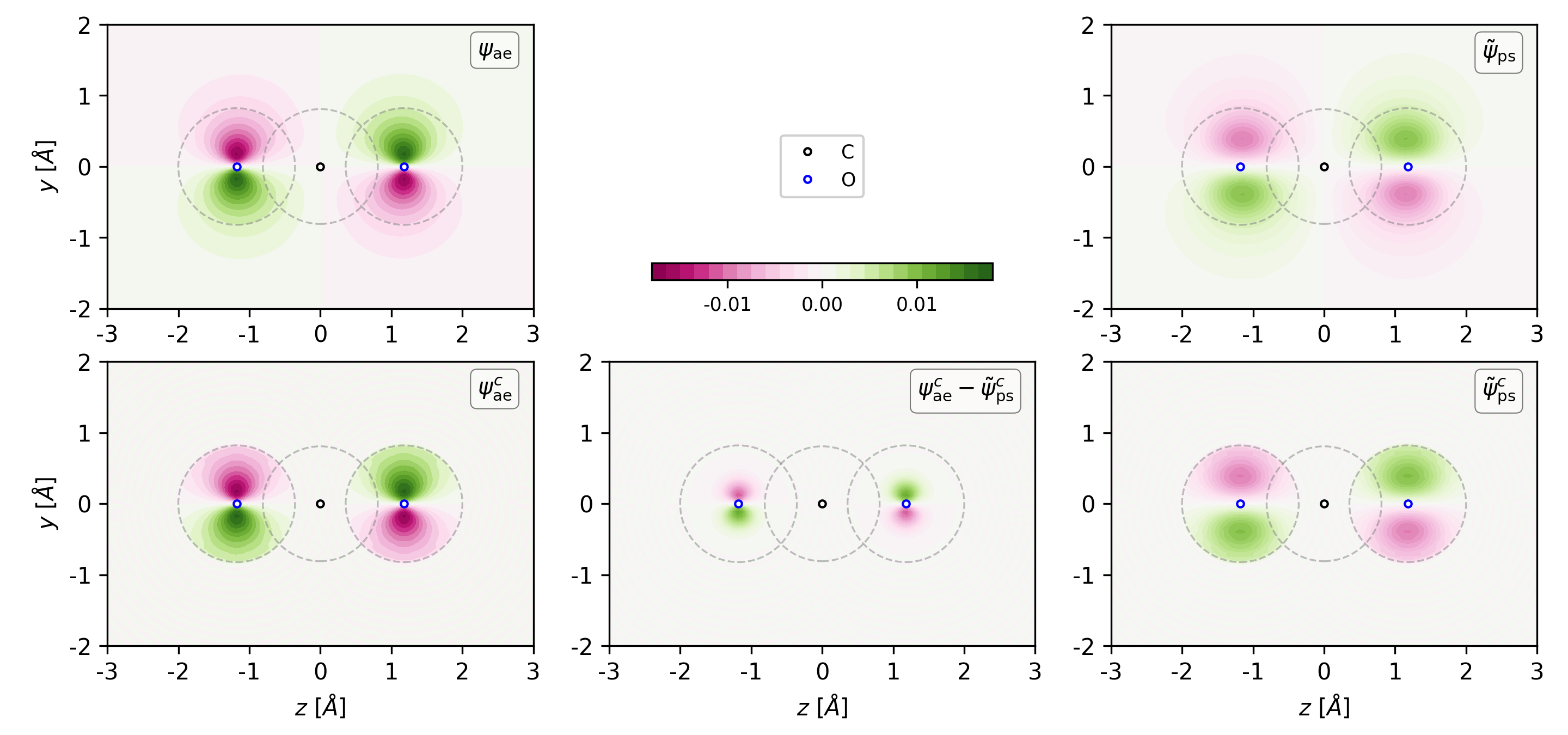
Figure 3. 2D plot of CO₂ HOMO orbital at x = 0 plane. The solid circles indicate the positions of the carbon and oxygen atoms while the dashed circles show the corresponding PAW sphere. The C-O bond length is 1.178 $\overset{˚}{A}$ while the PAW cutoff radius for C and O are 0.809 $\overset{˚}{A}$ and 0.822 $\overset{˚}{A}$ , respectively. The related files used to generate this figure can be found in examples of the VaspBandUnfolding package.
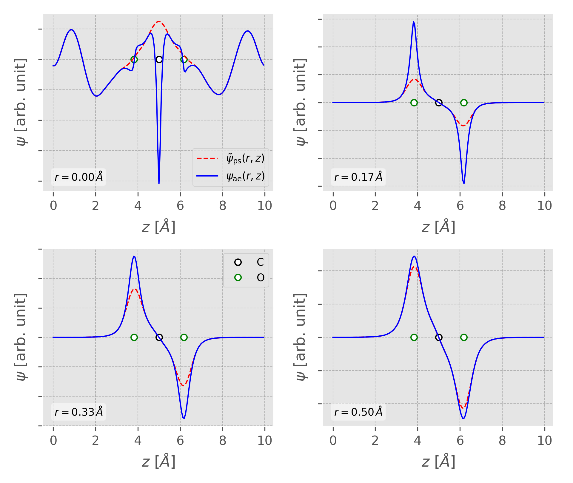
Wavefunctions $ψ (r, z)$ along the bond direction $z$ at different vertical distances $r$ .

Figure 4. Comparison of all-electron (blue solid line) and pseudo-wavefunction (red dashed line) of the CO₂ HOMO orbital, where $z$ is along the CO₂ bond direction and $r$ is the direction perpendicular to the CO₂ bond. The circles indicate the positions of the carbon and oxygen atoms. The related files used to generate this figure can be found in examples of the VaspBandUnfolding package.

Reference

Projector augmented-wave method ↩
Fourier Transform of Radial Functions ↩
pySBT: A python implementation of spherical Bessel transform (SBT) in O(Nlog(N)) time. ↩
Linear optical properties in the projector-augmented wave methodology ↩
From ultrasoft pseudopotentials to the projector augmented-wave method ↩ ↩²
In another VASP lecture note, 3-4 spherical Bessel functions are used in the expansion. ↩
As odd powers in r results in a kink in the functions at the origin, i.e. that the first derivatives are not defined at this point. ↩
Efficient pseudopotentials for plane-wave calculations ↩

PAW All-Electron Wavefunction in VASP

Introduction

AEWFC and PSWFC

Projector Function

Partial Waves

Constructing AEWFC

real-space approach

momentum-space approach

AEWFC & PSWFC of CO2 Orbital

Reference

Further Reading

Light-Matter Interaction and Dipole Transition Matrix

Band Unfolding Tutorial

VASP: Stacking-dependent Potential Energy Surface of Bilayer MoS2

Trending Tags

AEWFC & PSWFC of CO₂ Orbital

VASP: Stacking-dependent Potential Energy Surface of Bilayer MoS₂